Anomaly Detection

Last updated on Aug 3, 2020 Statistics

1 Point Anomaly Detection - Grubbs' test
2 Collective Anomaly Detection
- 2.1 Anomaly in timeseries - Seasonal Hybrid ESD algorithm
- 2.2 Distance-based Anomaly Detection
  - 2.2.1 Global Anomaly - Largest Distance
  - 2.2.2 Local Anomaly - LOF
3 Isolation Forest
- 3.1 Isolation Score

1 Point Anomaly Detection - Grubbs' test

Grubbs' test¹ is commonly used technique to detect an outlier in univariate problem, where normality assumption is required. It can be formualted as either one-side testing problem or two-sided testing problem.

The hypothesis test is defined as

$H_{0} : There are no outlier in the data set H_{1} : There is exactly one outlier in the data set .$ For two-sided testing, it tries to determine whether the observation with the largest absolute deviation is an outlier, where the test statistic is defined as

$G = \frac{max_{i} | X_{i} - \bar{X} |}{s},$ where the $\bar{X}$ is the sample mean and $s$ is the sample deviation.

Let's look at one simulated example.

set.seed(123)
simulated_data <- rnorm(100, 0, 1)
simulated_data_with_outliers <- c(simulated_data, c(3.5, -3.7))
# normality check
shapiro.test(simulated_data_with_outliers)

## 
##  Shapiro-Wilk normality test
## 
## data:  simulated_data_with_outliers
## W = 0.9804, p-value = 0.1344

Shapiro-Wilk normality test impiles the data is normally distributed. Now, let's performe the grubbs' test.

library(outliers)
grubbs.test(simulated_data_with_outliers, two.sided = TRUE)

## 
##  Grubbs test for one outlier
## 
## data:  simulated_data_with_outliers
## G = 3.65380, U = 0.86651, p-value = 0.01626
## alternative hypothesis: lowest value -3.7 is an outlier

The test result detecs the lowest value as an outlier.

Let's remove the -3.7 and performe the test again.

grubbs.test(head(simulated_data_with_outliers,101), two.sided = TRUE)

## 
##  Grubbs test for one outlier
## 
## data:  head(simulated_data_with_outliers, 101)
## G = 3.48190, U = 0.87755, p-value = 0.03378
## alternative hypothesis: highest value 3.5 is an outlier

Finally, let's remove two outliers altogether.

grubbs.test(head(simulated_data_with_outliers,100), two.sided = TRUE)

## 
##  Grubbs test for one outlier
## 
## data:  head(simulated_data_with_outliers, 100)
## G = 2.62880, U = 0.92949, p-value = 0.7584
## alternative hypothesis: lowest value -2.30916887564081 is an outlier

This impiles there are no outliers.

Grubbs' test is useful for identify the outliers of a small amount one at a time, but not suitable to detect a group of outliers.

2 Collective Anomaly Detection

2.1 Anomaly in timeseries - Seasonal Hybrid ESD algorithm

#  devtools::install_github("twitter/AnomalyDetection")
library(AnomalyDetection)
river <- read.csv("https://raw.githubusercontent.com/Rothdyt/personal-blog/master/static/post/dataset/river.csv")
results <- AnomalyDetectionVec(river$nitrate, period=12, direction = 'both', plot = T)

results$plot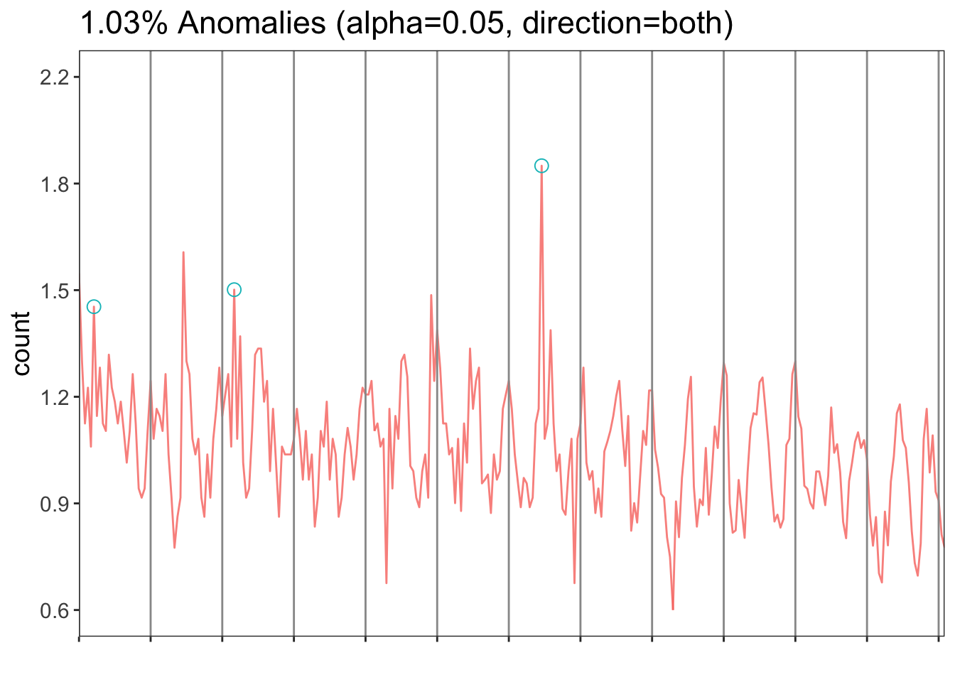

2.2 Distance-based Anomaly Detection

2.2.1 Global Anomaly - Largest Distance

Intuitively, the larger distance the more likely the point would be an outlier.

library(FNN)

## Warning: package 'FNN' was built under R version 3.4.4

furniture <- read.csv("https://raw.githubusercontent.com/Rothdyt/personal-blog/master/static/post/dataset/furniture.csv")
furniture_scaled <- data.frame(Height = scale(furniture$Height), Width = scale(furniture$Width))
furniture_knn <- get.knn(furniture_scaled, k = 5)
furniture_scaled$score_knn <- rowMeans(furniture_knn$nn.dist)
largest_idx <- which.max(furniture_scaled$score_knn)
plot(furniture_scaled$Height, furniture_scaled$Width, cex=sqrt(furniture_scaled$score_knn), pch=20)
points(furniture_scaled$Height[largest_idx], furniture_scaled$Width[largest_idx], col="red", pch=20)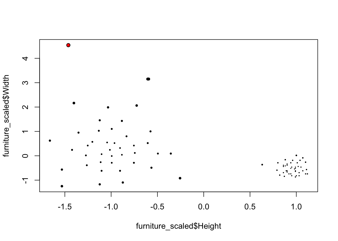

2.2.2 Local Anomaly - LOF

kNN is useful for finding global anomalies, but is less able to surface local outliers.

LOF is a ratio of densities:

LOF > 1 more likely to be anomalous LOF ≤ 1 less likely to be anomalous
Large LOF values indicate more isolated points

library(dbscan)
furniture_lof <- furniture[,2:3]
furniture_lof$score_lof <- lof(scale(furniture_lof), k=5)
largest_idx <- which.max(furniture_lof$score_lof)
plot(furniture_lof$Height, furniture_lof$Width, cex=sqrt(furniture_lof$score_lof), pch=20)
points(furniture_lof$Height[largest_idx], furniture_lof$Width[largest_idx], col="red", pch=20)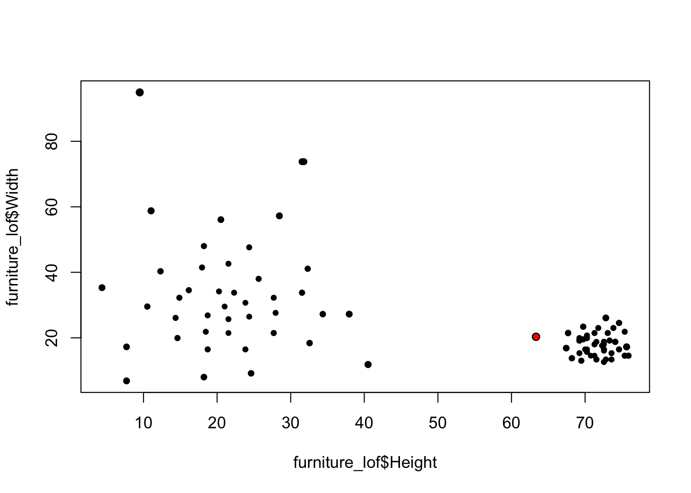

It's clear that, lof successfuly detects the local outlier.

3 Isolation Forest

Isolation Forest is built on the basis of decision trees;
To grow a decision tree, at each node, a feature and a corresponding cutoff value are randomly selected;
Intuitively, outliers are less frequent than regular observations and are different from them in terms of values, so outliers should be identified closer to the root of the tree with fewer splits. We use isolation score to characterize this.

3.1 Isolation Score

We need some quatity to define the isolation score²

Path Length: $h (x)$ of a point $x$ is measured by the number of edges $x$ traverses an iTree from the root node until the traversal is terminated at an external node.
Normalizing constant $c (n) = 2 H (n - 1) - (2 (n - 1) / n)$ , where $n$ is the number of samples to grow a tree and $H (i)$ is the harmonic number and it can be estimated by $l n (i) + 0.5772156649$ (Euler’s constant).

The isolation score $s$ of an sample $x$ is defined as $s (x, n) = 2^{- \frac{E (h (x))}{c (n)}},$ where the $E ()$ is the expectation of $h (x)$ .

Interpreting the isolation score:
Scores between 0 and 1
Scores near 1 indicate anomalies (small path length)

# devtools::install_github("Zelazny7/isofor")
library(isofor)
furniture <- read.csv("https://raw.githubusercontent.com/Rothdyt/personal-blog/master/static/post/dataset/furniture.csv")
furniture <- data.frame(Height = furniture$Height, Width = furniture$Width)
scores <- matrix(nrow=dim(furniture)[1])
for (ntree in c(100, 200, 500)){
  furniture_tree <- iForest(furniture, nt = ntree, phi=50)
  scores <- cbind(scores, predict(furniture_tree, furniture)) 
}
plot(scores[,3], scores[,4], xlab = "200 tress", ylab="500 tress")
abline(a=0,b=1)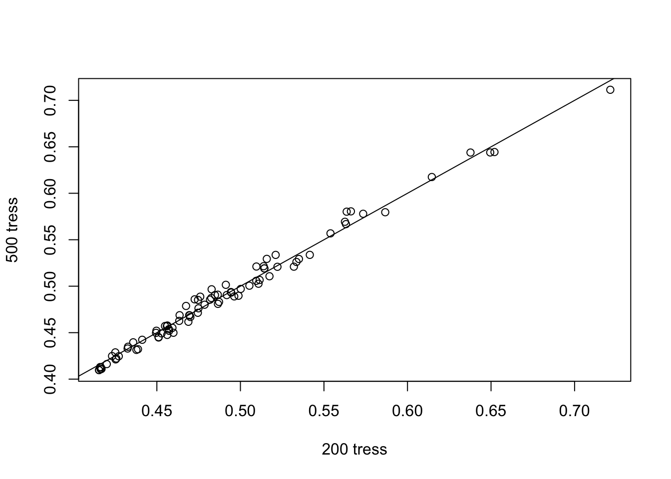

This graph is used to assess wheter the number of trees is enough for the isolation score to converge. From the graph above, we know that 200 tress are enough for us to identify the anomalies.

library(lattice)
furniture_forest <- iForest(furniture, nt = 200, phi=50)
h_seq <- seq(min(furniture$Height), max(furniture$Height), length.out = 20) 
w_seq <- seq(min(furniture$Width), max(furniture$Width), length.out = 20)
furniture_grid <- expand.grid(Width = w_seq, Height = h_seq)
furniture_grid$score <- predict(furniture_forest, furniture_grid)
contourplot(score ~ Height + Width, data = furniture_grid,region = TRUE)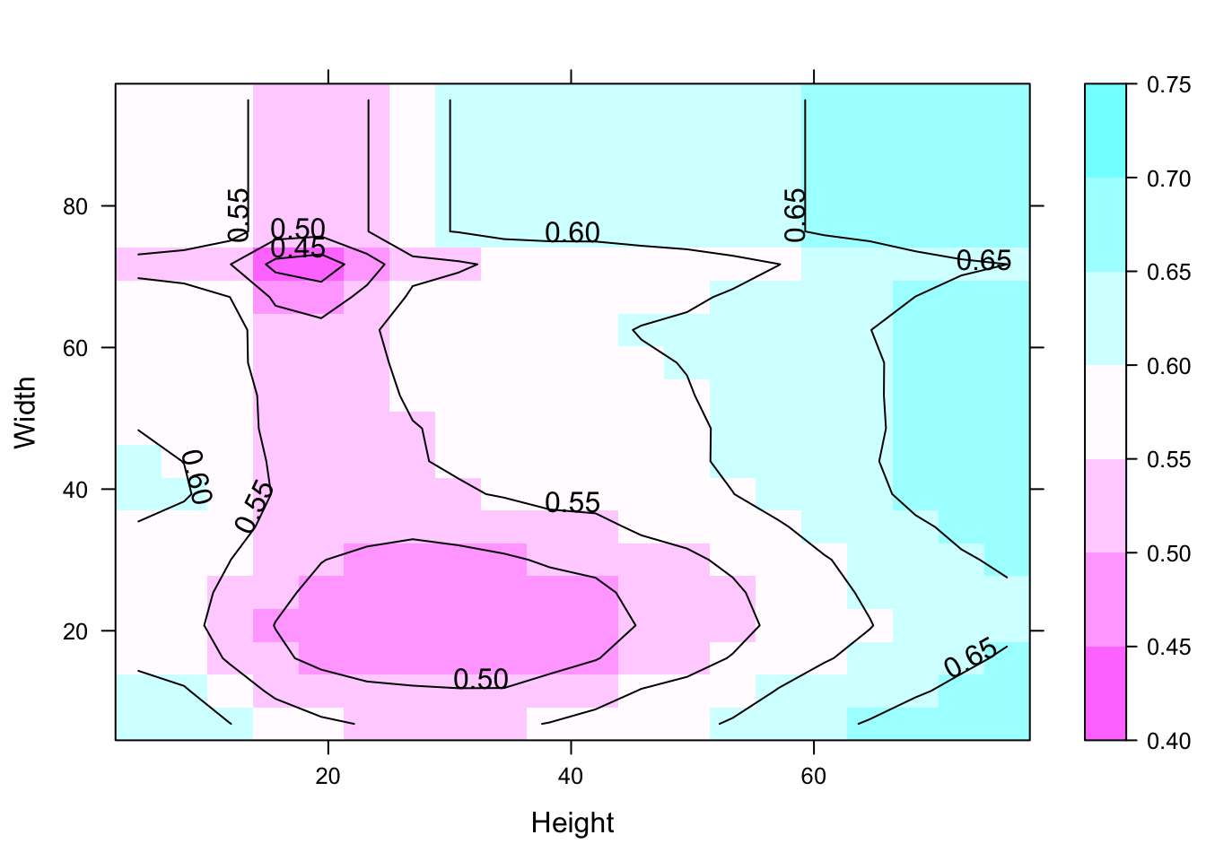

This contour graph used to identify the anomaly regions.

data-analysis