Problem description

Convergence Analysis

Theorem Suppose that $f$ is continuously differentiable over the set $X$ defined as above. Furthermore, suppose that for each $i$ and $x\in X$,

$$f(x_1,...,x_{i-1},\xi ,x_{i+1,....,x_m})$$

viewed as a function of $\xi$, attains a unique minimum ${\overline{x}}_i$ over $X_i$ and is monotonically non-increasing in the interval from $x_i$ to $\overline{\xi }$. Let $\{x_k\}$ be the sequence generated by the block coordinate method with Gauss-Seidel manner. Then, every limit point of $\{x_k\}$ is a stationary point.

PROOF

Let

$$z_i^k=(x_1^{k+1},...,x_i^{k+1},x_{i+1}^k,...,x_m^k)$$

By the nature of this algorithm, for all $k\ge 0$, we have following inequality

$$f(x^k)\ge f(z_1^k)\ge f(z_2^k)\ge ...\ge f(z_{m-1}^k)\ge f(x^{k+1})(\ast )$$

Since $\{x_k\}inX$, we can assume $\{x^{k_j}\}$ is the subsequence that converges to $\overline{x}=({\overline{x}}_1,..,{\overline{x}}_m)$.

Now we want prove that $\overline{x}$ is the stationary point of $f$.

From (*), we know that

$$f(z_1^{k_j})\le f(x_1,x_2^{k_j},...,x_m^{k_j})\mathrm{\forall }{x}_1\in X_1$$

Let $j\to +\mathrm{\infty }$, we derive

$$f(\overline{x})\le f(x_1,{\overline{x}}_2,...,{\overline{x}}_m)\stackrel{\mathrm{\Delta }}{=}h(x_1)\mathrm{\forall }{x}_1\in X_1$$

which implies that ${\overline{x}}_i$ is the minima of $h(x_1)$ on $X_1$. Using the optimality over a convex set, we conclude that

$$h^{\prime }({\overline{x}}_1)({\overline{x}}_1-x_1)\ge 0\iff (x_1-{\overline{x}}_1{)}^T{\mathrm{\nabla }}_{1}f({\overline{x}}_1)\ge 0x_1\in X_1$$

At this stage, if we can prove that $\{z_1^{k_j}\}$ converges to $\overline{x}$, we can show that

$$(x_2-{\overline{x}}_2{)}^T{\mathrm{\nabla }}_{2}f({\overline{x}}_2)\ge 0x_2\in X_2$$, since

$$f(z_1^{k_j})=f(x_1^{k_j+1},x_2^{k_j},x_3^{k_j},...,x_m^{k_j})\le f(x_1^{k_j+1},x_2,x_3^{k_j},...,x_m^{k_j})x_2\in X_2$$

Let $j\to +\mathrm{\infty }$, we derive

$$f(\overline{x})\le f({\overline{x}}_1,{\overline{x}}_2,{\overline{x}}_3,...,{\overline{x}}_m)\mathrm{\forall }{x}_2\in X_2$$

and

$$(x_2-{\overline{x}}_2{)}^T{\mathrm{\nabla }}_{2}f({\overline{x}}_2)\ge 0x_2\in X_2$$

(Note: Although $x_1^{k_j+1}$ may not in the sequence $\{x_1^{k_t}{\}}_{t\ge 1}$ ,which convergences to ${\overline{x}}_1$, but $\{z_1^{k_j}\}$ converges to $\overline{x}$, so its component $x_1^{k_j+1}$ converges to ${\overline{x}}_1$).

Furthermore, if we prove that for $i=1,2,...,m-1$,$\{z_i^{k_j}\}$ convergences to $\overline{x}$, then we have

$$(x_i-{\overline{x}}_i{)}^T{\mathrm{\nabla }}_{i}f({\overline{x}}_i)\ge 0x_i\in X_i$$

And thus $\overline{x}$ is a stationary point, since $(x-\overline{x}{)}^T\mathrm{\nabla }f(\overline{x})\ge 0$

By far, it remains to prove that $\{z_i^{k_j}\},\mathrm{\forall }i$ convergence to $\overline{x}$. First,we try to prove that $\{z_1^{k_1}\}$ convergence to $\overline{x}$.

Assume the contrary that $r^{k_j}=||z_1^{k_j}-x^{k_j}||$ doesn't convergence to 0. Let $s_1^{k_j}=(z_1^{k_j}-x^{k_j})/r^{k_j}$. Thus, $z_1^{k_j}=x^{k_j}+r^{k_j}{s}_1^{k_j}$ , $||r_{k_j}||=1$ and $s_1^{k_j}$ differs from 0 only along the first block-component. Since $\{s_1^{k_j}\}$ belong to a compact set and therefore without loss of generality, we assume $s_1^{k_j}$ convergences to ${\overline{s}}_1$.

Since $r^{k_j}>0$,we can find a $ϵ\in (0,1)$, such that $x^{k_j}+ϵs_1^{k_j}$ lies on the segment joining $x^{k_j}$ and $x^{k_j}+s_1^{k_j}=z_1^{k_j}$. Using the non-increasing property of $f$,we derive,

$$f(z_1^{k_j})\le f(x^{k_j}+ϵs_1^{k_j})\le f(x^{k_j})$$

Again, using (*), we conclude

$$f(x^{k_{j+1}})\le f(z_1^{k_j})\le f(x^{k_j}+ϵs_1^{k_j})\le f(x^{k_j})$$

Let $j\to +\mathrm{\infty }$, we derive $f(\overline{x})=f(\overline{x}+ϵ{\overline{s}}_1)$, which contradicts the hypothesis that $f$ is uniquely minimized when viewed as a function of the first block component. This contradiction establishes that $\{z_1^{k_1}\}$ convergence to $\overline{x}$.

Similarly, let $r_t^{k_j}=||z_t^{k_j}-z_{t-1}^{k_j}||$ for $t=2,3,...,m-1$ and using the same technique shown above, we finally prove that $\{z_i^{k_j}\},\mathrm{\forall }i$.

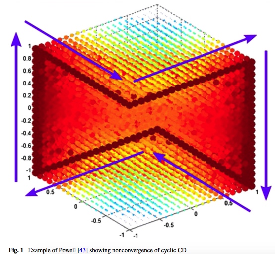
Powell's example

In ON SEARCH DIRECTIONS FOR MINIMIZATION ALGORITHMS, Power actually gives three examples that sequences generated by the algorithm discussed above do not convergence to stationary points once some hypothesis are not met.

• The first example is straightforward, However, the remarkable properties of this example can be destroyed by making a small perturbation to the starting vector $x^0$.

• The second example is not sensitive to either small changes in the initial data or to small errors introduced during the iterative process, for example computer rounding errors.

• The third example suggests that a function that is infinitely differentiable that also causes an endless loop in the iterative minimization method.

We here only presents the first example. Consider the following function

$$f(x,y,z)=-(xy+yz+zx)+(x-1{)}_{+}^2+(-x-1{)}_{+}^2+(y-1{)}_{+}^2+(-y-1{)}_{+}^2+(z-1{)}_{+}^2+(-z-1{)}_{+}^2$$

where

$$(x-c{)}_{+}^2=\{\begin{array}{l}0,x-c<0\\ (x-c{)}^2,x-c\ge 0\end{array}$$

Given the starting point $x_0=(-1-e,1+\frac{1}{2}e,-1-\frac{1}{4}e)$ and use block coordinate decent algorithm,and we update the variable in a manner of $x\to y\to z\to x...$ with

$$x_{k+1}^{\ast \ast }\leftarrow \text{sign}(y_k+z_k)[1+\frac{1}{2}|y_k+z_k|]$$

$$y_{k+1}^{\ast \ast }\leftarrow \text{sign}(x_{k+1}+z_k)[1+\frac{1}{2}|x_{k+1}+z_k|]$$

$$z_{k+1}^{\ast \ast }\leftarrow \text{sign}(x_{k+1}+y_{k+1})[1+\frac{1}{2}|x_{k+1}+y_{k+1}|]$$

We here present the first six steps of this case

This result implies that the sequence obtained by this algorithm can not converge to one single point since $x-coordinate$ change its sign as the even cycle and odd cycle alternate. Situations are similar for $y-coordinate$ and $z-coordinate$.

But $\{x_k\}$ has six sub-sequences which convergence to (1,1,-1), (1,-1,-1), (1,-1,1), (-1,-1,1),(-1,-1,1),(-1,1,1),(-1,1,-1) respectively.

Remark

1. A hint to derive the update formula:

   $$x\leftarrow \text{sign}(y+z)[1+\frac{1}{2}(y+z)]$$

   Indeed, derivates of $(x-1{)}_{+}^2$ and $(-x-1{)}_{+}^2$ are as follows respecively

   $$\frac{d(x-1{)}_{+}^2}{dx}=\{\begin{array}{l}2(x-1),x\ge 1\\ 0,x<1\end{array}\frac{d(-x-1{)}_{+}^2}{dx}=\{\begin{array}{l}2(-x-1),x\le -1\\ 0,x>-1\end{array}$$

   So for the univariate optimization problem, setting the derivate of $g(x)=f(x,y,z)$ to zero, we conclude

   $$\frac{\partial f(x,y,x)}{\partial x}=0\Rightarrow \{\begin{array}{l}x\ge 1:x=1+\frac{1}{2}(y+z)\\ -1<x<1:-(y+z)=0\\ x\le -1:x=-1+\frac{1}{2}(y+z)\end{array}$$

2. The gradient of $f(x,y,z)$ on this cyclic path, is $\mathrm{\nabla }f(x,y,z)=(-y-z,-x-z,-x-y)$ and $||\mathrm{\nabla }f(x,y,z)|{|}_1=2$

3. This example is unstable with respect to small perturbations. Small changes in the starting point $x_0=(-1-e,1+\frac{1}{2}e,-1-\frac{1}{4}e)$ or smal errors in the numbers that are computed during the calculation will destroy the cyclic behavior.

   It's s clear the choice of perturbations $e$ plays a key role. Say, $x_0=(-1-e_1,1+e_2,-1-e_3)$ and we have $e_k=\frac{1}{2}(e_{k-2}-e_{k-1})$

   cycle/totall iteration	x	y	z
   1/1	1+$e_4$	1+$e_2$	-1-$e_3$
   1/2	1+$e_4$	-1-$e_5$	-1-$e_3$
   1/3	1+$e_4$	-1-$e_5$	1+$e_6$
   2/4	-1-$e_7$	-1-$e_5$	1+$e_6$
   2/5	-1-$e_7$	1+$e_8$	1+$e_6$
   2/6	-1-$e_7$	1+$e_8$	-1-$e_9$
   ...	...	...	...

   To preserve the cyclic behavior , we have to make sure that $e_{k-2}>e_{k-1}$

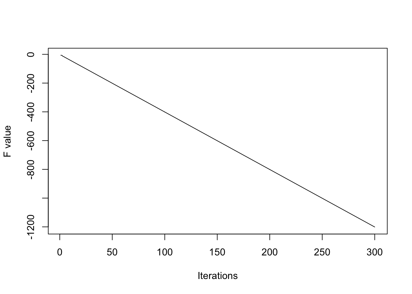
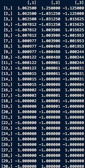
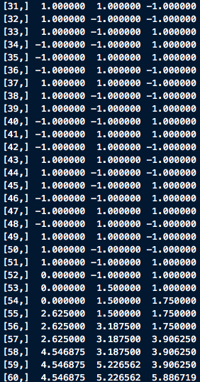
   And in practice, when we do some numerical tests, we shall find that, this theoretically-existed endless loop actual breaks down due to the rounding errors. A brief illustration is given below. In this experiment, loop ends at the 52 steps.

   
   

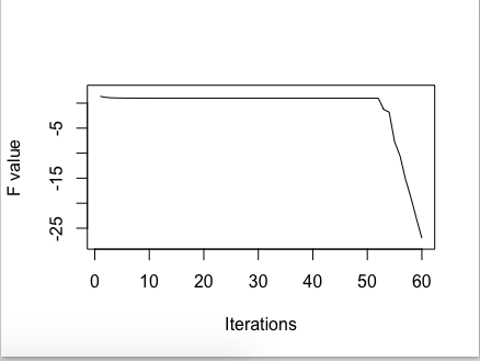
4. As
   $$\frac{\partial f(x,y,x)}{\partial x}=0\Rightarrow \{\begin{array}{l}x\ge 1:x=1+\frac{1}{2}(y+z)\\ -1<x<1:-(y+z)=0\\ x\le -1:x=-1+\frac{1}{2}(y+z)\end{array}$$

   suggests that, when $-1<x<1$, the choice of $x$ is arbitrary and we set $x^{\ast }=0$ in the case above. So the uniqueness requirement is violated. It turns out that the six vertices are even not the stationary points.

   For example, at point $\overline{x}=(1,1,-1)$, $\mathrm{\nabla }f(\overline{x})=(0,0,-2)$ and for any ponit $x$ in the unit cubic $(x-\overline{x}{)}^T\mathrm{\nabla }f(\overline{x})\le 0$. Say, $x=(0.9,0.9,-0.9)$, $(x-\overline{x}{)}^T\mathrm{\nabla }f(\overline{x})=-0.2<0$

   Actually, as in the proof of Theorem, we prove that $\{z_1^{k_j}\}$ converges to $\overline{x}$, where $\overline{x}$ is the limit point of $\{x^{k_j}\}$. But in this example, the limit point of $\{z_1^{k_j}\}$ is (1,1,-1) while the limit point of $\{x^{k_j}\}$ is either (-1,1,-1) or (1,-1,1). So the requirement of uniqueness is not met.

R codes for numerical experiments

####################
### Function for test ###
####################

PowellE1<-function(xstart,cycles,fig=T){
  #######function part ##############
  UpdateCycle<-function(x){
    Sign<-function(x){
      if (x>0){
        return(1)
      }else{
        if (x<0){
          return(-1)
        }else{
          return(0)
        }
      }
    }
    x.new<-c()
    x.new[1]<-Sign(x[2]+x[3])*(1+0.5*abs(x[2]+x[3]))
    x.new[2]<-Sign(x.new[1]+x[3])*(1+0.5*abs(x.new[1]+x[3]))
    x.new[3]<-Sign(x.new[1]+x.new[2])*(1+0.5*abs(x.new[1]+x.new[2]))
    cycle<-matrix(c(x.new[1],x[2],x[3],x.new[1],x.new[2],x[3],x.new[1],x.new[2],x.new[3]),
                  ncol=3,byrow=T)
    return(cycle)
  }
  
  fpowell<-function(x){
    
    PostivePart<-function(x){
      ifelse(x>=0,x,0)
    }
    
    fval<-(-(x[1]*x[2]+x[2]*x[3]+x[1]*x[3]))+
      PostivePart(x[1]-1)^2+PostivePart(-x[1]-1)^2+
      PostivePart(x[2]-1)^2+PostivePart(-x[2]-1)^2+
      PostivePart(x[3]-1)^2+PostivePart(-x[3]-1)^2
    return(fval)
  }
  ############ operation part ################
  x.store<-matrix(ncol=3,nrow=cycles*3+1)
  x.store[1,]<-xstart
  for (i in seq_len(cycles)){
    x.store[(3*i-1):(3*i+1),]<-UpdateCycle(x.store[3*i-2,])
  }
  x.store<-x.store[-1,]
  fval<-rep(0,cycles*3)
  
  for(i in seq_len(cycles*3)){
    fval[i]<-fpowell(x.store[i,])
  }
  fval<-as.matrix(fval)
  
  if (fig==T){
    plot(fval,ylim=c(min(fval)-1,max(fval)+1),type="l",xlab="Iterations",ylab = "F value")
  }
  r<-list()
  r$x.iterate<-x.store
  r$fval<-fval
  return(r)
}


##################
#### Test 1 ########
##################


perturb<-0.5
xstart<-c(-1-perturb,1+0.5*perturb,-1-0.25*perturb)
cycles<-20

r<-PowellE1(xstart,cycles,fig=T)

##################
#### Test 2 ########
##################

perturb<-0.5
xstart<-c(-1-perturb,1+0.5*perturb,-1-0.25*perturb)
cycles<-20

r<-PowellE1(xstart,cycles,fig=T)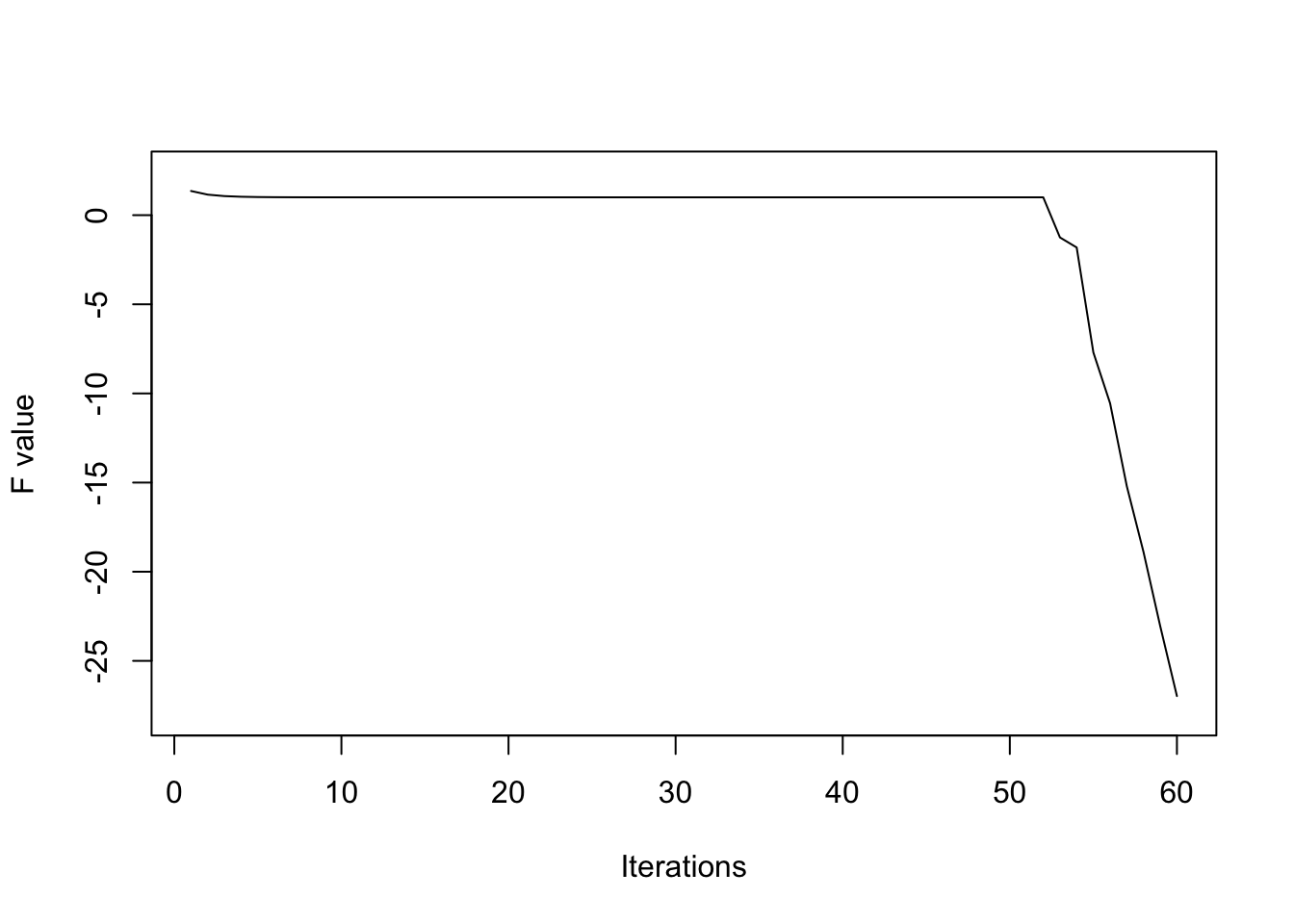

##################
#### Test 3 ########
##################

xstart<-c(3,2,1)
cycles<-100

r<-PowellE1(xstart,cycles,fig=T)